AnalyzeCellCount
AnalyzeCellCount[MicroscopeData]⟹CellCountObject
counts the number of cells and their area and morphology given a microscope data object according to the type of cells in the aquired image. The function performs adjustment of image specification such as brightness and contrast and performs image segmentation.
AnalyzeCellCount[ImageFiles]⟹CellCountObject
counts the number of cells and measures the cell size and morphology by first adjusting the image specifications such as brightness and contrast and then performing image segmentation.
Details
- To view examples in the "Additional Examples" section of this helpfile, please evaluate the "Example Setup" section and then re-evaluate the additional example cells.
- There are three major algorithms used for segmentation. The default algorithm is optimized for well-separated cells or cell clusters.
- If MeasureConfluency->True, an algorithm is used on the basis of the paper "A Method for Quick, Low-Cost Automated Confluency Measurements" by Topman et al., Microsc. Microanal. 17, 915-922, 2011.
- The method detects the denuded areas in a micrograph of a culture based on standard deviation of pixel intensities, where low SD values indicate absence of cells and high SD values correspond to areas populated by cells.
- Note that the number of cells that is given as the output for a confluency measurement analysis is just the total number of disconnected components and is not the number of each individual cells within the segmented cell cluster.
- Two window sizes are used per each image: "big" window and "small" window, to achieve arrays of coarse and fine homogeneity measures.
- Threshold values are binarization can be determined for a given cell type through iterative visual inspection of detected denuded areas in the final output image and increased if the denuded areas are smaller than desired, or decreased otherwise.
- Opening is performed which is the operation of erosion followed by dilation, resulting in the removal of small isolated areas. Next morphological closing is done which is the operation of dilation followed by erosion, which results in the filling of small isolated "holes" in the image.
- If Hemocytometer->True, another algorithm is used which is similar to that of "Automated Cell Counting and Characterization" technical report by Janice Lai.
- The region of interest is chosen by a pair position index where {1,1} indicates lower left hemocytometer square and {n,n} indicates the top right square.
- In this algorithm, the background grid is first removed and then a standard segmentation algorithm is performed to find the cells.
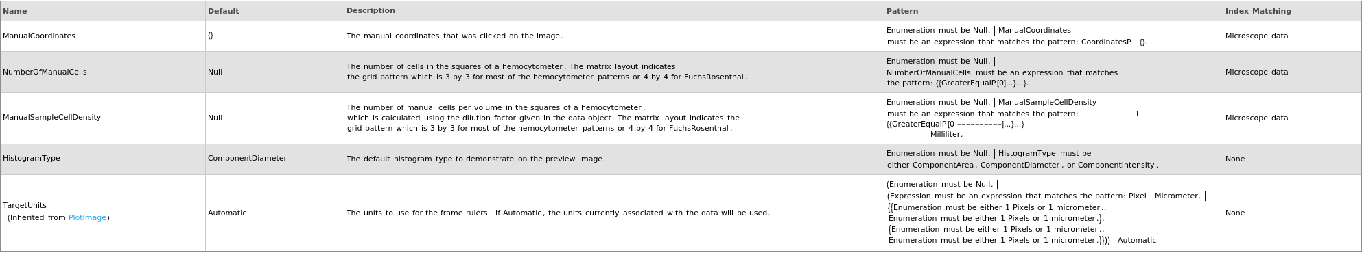
Input

Output

Confluency Measurement Options

Image Processing Options
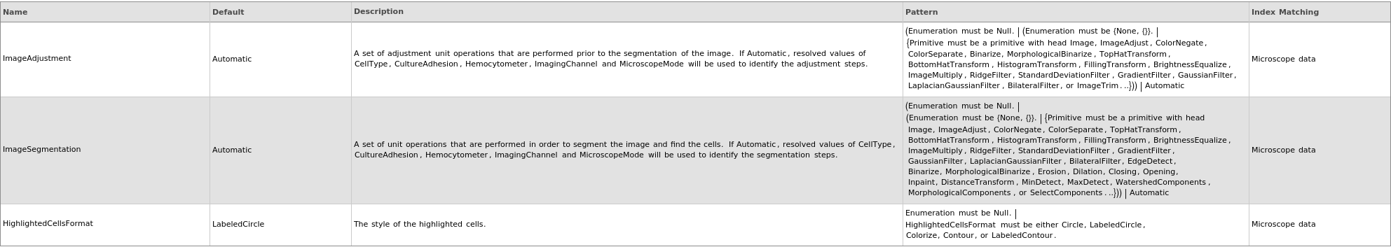
Image Selection Options

Output Processing Options
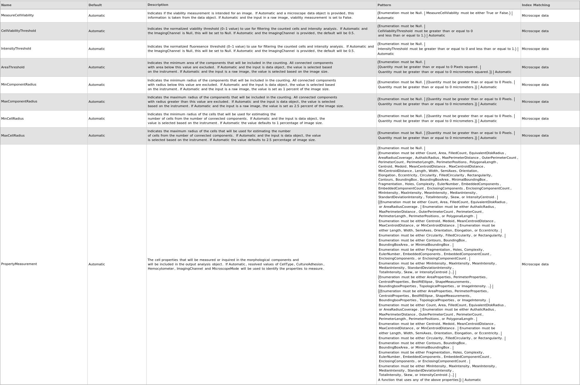
Property Measurement Options
Source Specifications Options
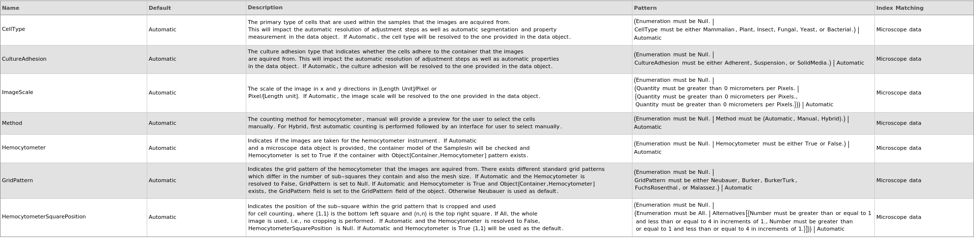
Method Options
Examples
open allclose allBasic Examples (5)
Confluency measurement using a short-hand notation, MeasureConfluency->True:
Count cell numbers for a hemocytometer images stored in a microscope data object and selecting all steps automatically:
Measure the viability of the cells from the colored image:
Segmentation of tissue culture cells using the default algorithm:
Visualize the area covered by cells which is used for confluency measurement:
Additional Examples (17)
Confluency measurement for multiple sites (1)
Confluency measurement steps (4)
A: The adjustment only contains brightening the image by two levels (each pixel intensity value increased by twice its pixel intensity value):
B: For the segmentation, we perform standard deviation filter to detect the more homogenous regions which are the cell free medium:
C: We perform the denuded area (cell-free zone) detection with two standard deviation sizes and call them small and big window: 1- standard deviation filter with a small window, 2- binarize the image using the small window filtered image, 3- standard deviation filter using a big window, 4- binarize the image using the big window filtered image, 5- dilate the binarized image with big window:
D: Finally, we determine the intersect of the cellular regions to indicate our final culture cell area and will perform a subsequent closing and opening to remove any holes and very small components: 1- standard deviation filter with a small window, 2- binarize the image using the small window filtered image, 3- standard deviation filter using a big window, 4- binarize the image using the big window filtered image, 5- dilate the binarized image with big window, 6- find the intersect of the dilated image with the small window binaized, 7- perform closing followed by opening with the intersect result:
Hemocytometer processing steps (4)
A: The adjustment steps are: 1- increasing the brightness of the image (given our camera setup the images are a little dark) and 2- trimming the image to select a sepecific square in the hemocytometer grid which depending on the type of the grid, is a pair of number {r,c} where r and c are between 1-3 or 1-4. In this case we are selecting square position {1,3}. The pixel coordinates can be determined by first plotting the input like PlotImage[myCloudFile]:
B: As for the standard segmentation procedure, we perform: 1- edge detection for the adjusted image so we will detect the contours of all components, 2- we close the detected lines (all circles) using Closing primitive which calls mathematica's Closing, 3,4- We perform dilation and erosion with the same kernel so for the detected components any holes will be filled remove any extremely small component will be removed:
C: After we find all components we need to remove the hemocytometer grid lines. For that we first use ridge filter to detect the grid lines and then binarize and finally remove the detected lines: 5- Use RidgeFilter to further use to find the mask (background grid) and ImageAdjust ing the result, 6- MorphologicalBinarize the result of ridge filter with a low threshold (0.05-0.5) to find the background grid mask, 7- Remove the background grid using Inpaint with the method Diffusion which is a compromise between time and quality:
D: Finally after removing the background grid lines, we use a standard process to avoid any overlap between the cells. This is done by first finding the distance of the cell boundary relative to their centers and then using watershed algorithm: 8- Find the distance transform which normalize the pixels according to their distance to edges of black and white boundary, 9- Find the maximum of the distance transform which indicates the centers of the components, 10- Find the regions of rapid pixel value change with gradient filter to indicate the regions associated with the components, 11- Finally perform the watershed algorithm on the result of the gradient filter with the marker set as the result of MaxDetect:
Interactive apps (2)
Neat examples for cell segmentation (5)
A: Segmenting the cells that are stained in one channel:
B: Standard segmentation of red blood cells taken from the mathematica guide pages:
C: Analyzing the deformation and morphology of the detected RBCs. We extract echinocytes cells by selecting cells of a certain size that exhibit tentacles of more than 5% of their total area:
Segmentation of Epifluorescence channel of Mammalian, HeLa-dsRed/GFP model cells:
Segmentation of small sparse tissue culture cells using the default algorithm:


